Sample Size
A revision of the slides will be available soon.
Exercise 1. Interpretation of a clinical study
Consider the following abstract reporting a clinical trial of reducing mortality by peripheral perfusion compared to lactate among patients in intensive care with septic shock.
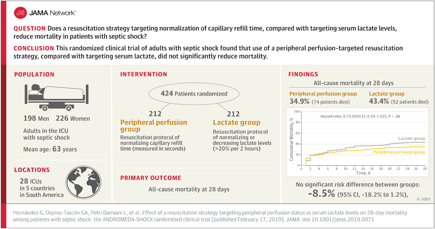
- What was the mortality rate in the treatment arm? In the control arm?
- What was the estimate for treatment effect?
- What was its confidence interval? (check our understand of 95% CI)
- What conclusion did the authors/journal draw? Why?
- What conclusions do you draw from this trial?
- If you or a loved one was in septic shock, which treatment would you prefer?
- Would you allow yourself to be randomised to these treatments in a future trial?
Exercise 2. How big should a study to estimate a proportion be?
Consider a study to estimate the prevalence of detectable virus in the stoll samples of COVID patients.
We can think about the sample size required in terms of the precision that the study needs to have
Suppose we recruited 10 patients, and found two positive samples. We can use binom.test in R to find the estimate and its 95% confidence interval.
Adapt the code to answer the following questions (leave notes in the code box if you like but remember these won’t be saved):
- What would be the confidence interval if we recruited 100 participants and found 20 positive samples?
- Suppose we expect the prevalence to be about 20%. How many samples will we need to estimate the prevalence to within +-5 percentage points.
- What if the prevalence was only 10%?
- How many samples should we collect for this study?
- Based on this study, what do we need to think about when deciding on a sample size?
Exercise 3. How big should a study to estimate a mean difference be?
We are interested in the number of mice needed to test the effect of supplement on fecal alpha diversity.
First we’ll explore replications of a single study, to revise our understanding of hypothesis tests, think about the interpretation of p-values and meaning of statistical power.
This first code block simulates a study, and generates a dataset. Choose any number for the seed, this will ensure that we all get independent runs of the experiment!
Look at the assumptions we need to make to simulate the dataset.
Next we can make beeswarm graph with a t-test to compare means:
Calculate the mean and standard deviation by group, run a t-test.
Lets stop here to make sure that we completely understand the t-test result.
Lets pause here to answer the following questions:
- How precise was the your initial effect estimate with 10 mice per group?
- How does this change with increasing sample size?
Reproducibility of the study, implication for power
To understand what the sampling distribution of our estimator is, and to better understand the likely reproducibility of this study, we can run a large number of simulations:
Questions for discussion:
- How reliable was the p-value across experiments?
- Did the experiments agree or disagree with respect to the efficacy of the treatment?
- How many mice would be ‘enough’ to reliably detect the effect that we introduced?
- How many mice would be enough to make a power of 80% ?
- How does this change if we change the size of the effect?
- How does this change if the mice become more variable?
Implications for ‘running a study many times’
As we’ve seen, p-values are not reliable. It is expected that given the same study design, sometimes you’ll get a significant difference and sometimes not.
This is a consequence of the variability of the experimental units, and does not represent a failure of the system or changing conditions in
So there is little value in repeating a study (say) three times and hoping for agreement.
If we had that resource then, it would be better to create one larger study, with blocks if necessary.
The graph below shows how the precision would increase if we had pooled results from repeats instead of trying to interpret each individually.
Exercise 4 - What is statistical power?
Check our understanding of the following terms
- What does it mean if an experiment has a power of, say, 80%?
- What is an ‘under-powered’ study?
- What would you learn from an underpowered study?
- How would you know if a study that you are reading was under-powered?
Exercise 5 – Logic of statistical inference
Why do scientists ignore sample size issues?
In my experience, we often have this paradigm for our statistical analyses:
- Do experiment
- Do analysis
- If p>0.05 – we have proved there is no effect,
- if p<0.05 – we have proved there is an effect
What’s wrong with this logic? Can you correct it?
Exercise 6. Using the pwr package to find sample size analytically
We will use a simple parallel group study to investigate this.
We believe from prior work that the within-group standard deviation for mouse alpha diversity is 1.
Use the pwr function to answer the following questions:
- Suppose we wanted our experiment to reliably detect an effect of 0.5 units, should it exist. How many mice would we need?
- If we could only afford to use ten mice per group, what would be the smallest effect size that we could detect?
- What is the power to detect a difference of 0.5 units, given that we only have ten mice per group.
- Remember we might not get data from all ten mice that were included. If only 80% are expected to survive and give usable data, would would the power be?
- How many mice would Mead’s resource equation suggest that we use?
- What would be the smallest detectable effect with this number?
Exercise 8. Sample size for comparing two proportions
Suppose we are interested in comparing an event incidence rate between two independent groups.
We expect in our model that 50% of the participants will develop the outcome. We expect our intervention will lower this to 20% percentage points. How many participants would we need to be able to detect this difference?
Now adapt the code to check how many participants would be needed to detect a difference between 50% and 40%.
Worked Example: Effective sample size with clustered data
Consider an observational study in which retinal nerve fibre layer thickness (RNFL) is compared between patients with or without rheumatoid arthritis.
Patients are to be randomly sampled from their respective populations, and each patient has a measurement taken in their left and their right eye.
How should we analyse this data, what are the implications if of using the wrong model, and what are the implications for power and sample size? How much extra information do we get from measuring the second eye in each participant?
First we’ll set up the simulation study:
It is valuable to plot the data to check the extent of the correlation between the eyes
Can we assume that eyes are independent observations in the analysis?
We could treat eyes as technical replicates, and take the average for each participant before running the t-test.
This is OK, we now have one measure per person, and each person was sampled independently.
So did we get any benefit from using two eyes instead of one, even though our sample size was still the same?
Yes, because of the repeated measurement our data for each person became less variable.
Compare the standard deviations if we used the left eye only compared to the aggregated data:
The relative increase in precision depends on how much of the overall variation is found within eyes vs between eyes. We set this above with the ICC (intraclass correlation coefficient). Here we set ICC=0.5.
We can show that the effective sample size using two eyes is
\[ N\times\frac{2}{1+\text{ICC}} \]
which in this case is \(1.33 \times N\)
So by using both eyes in this case we effectively increase the sample size by 30%.
A general formula for the effective sample size, for clusters of more than two (say mice within cages, is)
\[ N_{\text{Eff}} = N\times\frac{m}{1+(m-1)\times\text{ICC}} \] Where \(N\) is the number of units, and \(m\) is the number of clusters.
So suppose we allocated a treatment to mice, and they have a shared outcome such that the intra-class correlation is about 0.3. This might be typical for microbiome measures, stress responses, inflammatory responses etc. Then the effective sample size increases with the number of animals as follows:
This adds an extra complication to a sample size calculation, but you make reasonable assumptions based on prior work regarding what the ICC might be. In any case, simply assuming that mice are independent could lead you to vastly over-estimate the power of your study.
Clearly in terms of numbers, having fewer mice per cage is the most efficient, but optimising a sample size and a layout in this case (number of cages, number of mice per cage) depends also the relative cost of cages vs animals, and you will be limited by ethical and practical constraints.
For a full discussion see:
Randomising treatments within clusters
A converse situation arises if we can randomise eyes independently to treatments. In this case the unit of experiment is the eye, but we get the added benefit that we can remove the between-person variance from the analysis, since every person contributes one treated and one control eye.
If we plot the outcome with the individual participants identified, we should see that the effect of the treatment is more obvious, because the between-participant variation becomes irrelevant.
So here, instead of losing power, because we can randomise within the clusters we gain power. If we had to treat the individual and not the eye we would be randomising the clusters themselves, which would cost us power.
The effective sample size given N individuals, if we can randomise two treatments within an individual, is given by:
\[ N_\text{eff}=N\times\frac{2}{1-\text{ICC}} \]
Where \(N\) is the number of individuals. Now as the ICC goes up, the effective sample size also increases.
A similar logic applies to cross-over vs parallel group human trials. With an ICC of 0.5, then a parallel group study of, say, 100 individuals per group (total 200 individuals), would only require 50 individuals in total (100 eyes) if we can compare both treatments within each person.
Whether this is practically possible depends on the nature of the intervention and the experimental units themselves.