Iris dataset analysis walkthrough

Author

George Savva, QIB

Published

January 1, 2024

This file is intended as a summary of some of the important features discussed during the ‘R for Statistics’ training course.

The aspects covered are:

Loading data from csv files
Descriptive statistics
Graphing with base R and ggplot
Simple linear modelling with continuous outcomes, and categorical and continuous predictors

I do not include model diagnostics, nor data wrangling with tidyverse here. These are important topics that are introduced in the individual session worksheets.

1 Loading and describing data.

Load a package we will need:

library(ggplot2) # ggplot is for making publication quality graphs

Load data from a csv file using read.csv

iris <- read.csv("iris.csv")

Get some statistics on the structure of the dataset to make sure it’s all read in OK.

nrow(iris)

[1] 150

str(iris)

'data.frame':   150 obs. of  6 variables:
 $ X           : int  1 2 3 4 5 6 7 8 9 10 ...
 $ Sepal.Length: num  5.1 4.9 4.7 4.6 5 5.4 4.6 5 4.4 4.9 ...
 $ Sepal.Width : num  3.5 3 3.2 3.1 3.6 3.9 3.4 3.4 2.9 3.1 ...
 $ Petal.Length: num  1.4 1.4 1.3 1.5 1.4 1.7 1.4 1.5 1.4 1.5 ...
 $ Petal.Width : num  0.2 0.2 0.2 0.2 0.2 0.4 0.3 0.2 0.2 0.1 ...
 $ Species     : chr  "setosa" "setosa" "setosa" "setosa" ...

Extract single variables (vectors) from the dataset

iris$Sepal.Length

  [1] 5.1 4.9 4.7 4.6 5.0 5.4 4.6 5.0 4.4 4.9 5.4 4.8 4.8 4.3 5.8 5.7 5.4 5.1
 [19] 5.7 5.1 5.4 5.1 4.6 5.1 4.8 5.0 5.0 5.2 5.2 4.7 4.8 5.4 5.2 5.5 4.9 5.0
 [37] 5.5 4.9 4.4 5.1 5.0 4.5 4.4 5.0 5.1 4.8 5.1 4.6 5.3 5.0 7.0 6.4 6.9 5.5
 [55] 6.5 5.7 6.3 4.9 6.6 5.2 5.0 5.9 6.0 6.1 5.6 6.7 5.6 5.8 6.2 5.6 5.9 6.1
 [73] 6.3 6.1 6.4 6.6 6.8 6.7 6.0 5.7 5.5 5.5 5.8 6.0 5.4 6.0 6.7 6.3 5.6 5.5
 [91] 5.5 6.1 5.8 5.0 5.6 5.7 5.7 6.2 5.1 5.7 6.3 5.8 7.1 6.3 6.5 7.6 4.9 7.3
[109] 6.7 7.2 6.5 6.4 6.8 5.7 5.8 6.4 6.5 7.7 7.7 6.0 6.9 5.6 7.7 6.3 6.7 7.2
[127] 6.2 6.1 6.4 7.2 7.4 7.9 6.4 6.3 6.1 7.7 6.3 6.4 6.0 6.9 6.7 6.9 5.8 6.8
[145] 6.7 6.7 6.3 6.5 6.2 5.9

Note that R is case sensitive so this does not work:

iris$sepal.length

NULL

Get individual elements if we want to.

iris$Sepal.Length[1]

[1] 5.1

Get the 2nd, 4th and 6th elements (extract a subset by position)

iris$Sepal.Length[c(2,4,6)]

[1] 4.9 4.6 5.4

Get the 10th to the 20th elements of the vector

iris$Sepal.Length[10:20]

 [1] 4.9 5.4 4.8 4.8 4.3 5.8 5.7 5.4 5.1 5.7 5.1

By default, Species is read as a string (because the option stringsAsFactors is set to FALSE by default).
So if we want to use Species as a categorical variable we have to convert it into a ‘factor’.

iris$Species <- factor(iris$Species)

We can use the default plotting system to make a quick plot, but it’s a bit ugly!

plot(iris, col=iris$Species)

Demonstration of using the base hist function if we want a quick histogram

iris$Sepal.Width |> hist(breaks=20)

Summary does different things depending on what kind of object is passed to it.

summary(iris)

       X           Sepal.Length    Sepal.Width     Petal.Length  
 Min.   :  1.00   Min.   :4.300   Min.   :2.000   Min.   :1.000  
 1st Qu.: 38.25   1st Qu.:5.100   1st Qu.:2.800   1st Qu.:1.600  
 Median : 75.50   Median :5.800   Median :3.000   Median :4.350  
 Mean   : 75.50   Mean   :5.843   Mean   :3.057   Mean   :3.758  
 3rd Qu.:112.75   3rd Qu.:6.400   3rd Qu.:3.300   3rd Qu.:5.100  
 Max.   :150.00   Max.   :7.900   Max.   :4.400   Max.   :6.900  
  Petal.Width          Species  
 Min.   :0.100   setosa    :50  
 1st Qu.:0.300   versicolor:50  
 Median :1.300   virginica :50  
 Mean   :1.199                  
 3rd Qu.:1.800                  
 Max.   :2.500

summary(iris$Sepal.Width)

   Min. 1st Qu.  Median    Mean 3rd Qu.    Max. 
  2.000   2.800   3.000   3.057   3.300   4.400

summary(iris$Species)

    setosa versicolor  virginica 
        50         50         50

We can do a statistical test using two variables. (Although this association is better tested using lm as below)

cor.test(iris$Sepal.Length, iris$Petal.Width)


    Pearson's product-moment correlation

data:  iris$Sepal.Length and iris$Petal.Width
t = 17.296, df = 148, p-value < 2.2e-16
alternative hypothesis: true correlation is not equal to 0
95 percent confidence interval:
 0.7568971 0.8648361
sample estimates:
      cor 
0.8179411

Find the minimum sepal width

min(iris$Sepal.Width)

[1] 2

Tabulate the species to find the number of observations for each

table(iris$Species)


    setosa versicolor  virginica 
        50         50         50

2 Graphing

Make a histogram with red bars

hist(iris$Sepal.Length, col="red")

To quickly demonstrate the formula interface we made a (not very nice) boxplot.

boxplot( Petal.Length ~ Species , data=iris)

Could we have done this with the native pipe?
This doesn’t work (because if the arguments are unnamed iris needs to be the second argument)

iris |> boxplot(Petal.Length ~ Species)

But either of these two lines does work:

iris |> boxplot(Petal.Length ~ Species , data=_)
iris |> boxplot(data=_ , Petal.Length ~ Species )

We can make a much nice boxplot using ggplot2. Make sure you understand what each of these lines does!

iris |> ggplot() + 
  aes(x=Species , y=Petal.Length, fill=Species) + 
  geom_boxplot() + 
  ggtitle("Petal length by Species") + 
  theme_bw() + 
  scale_y_log10(breaks=c(1,2,3,4,5,6,7,8,9,10)) + 
  labs(y="Petal length (cm)")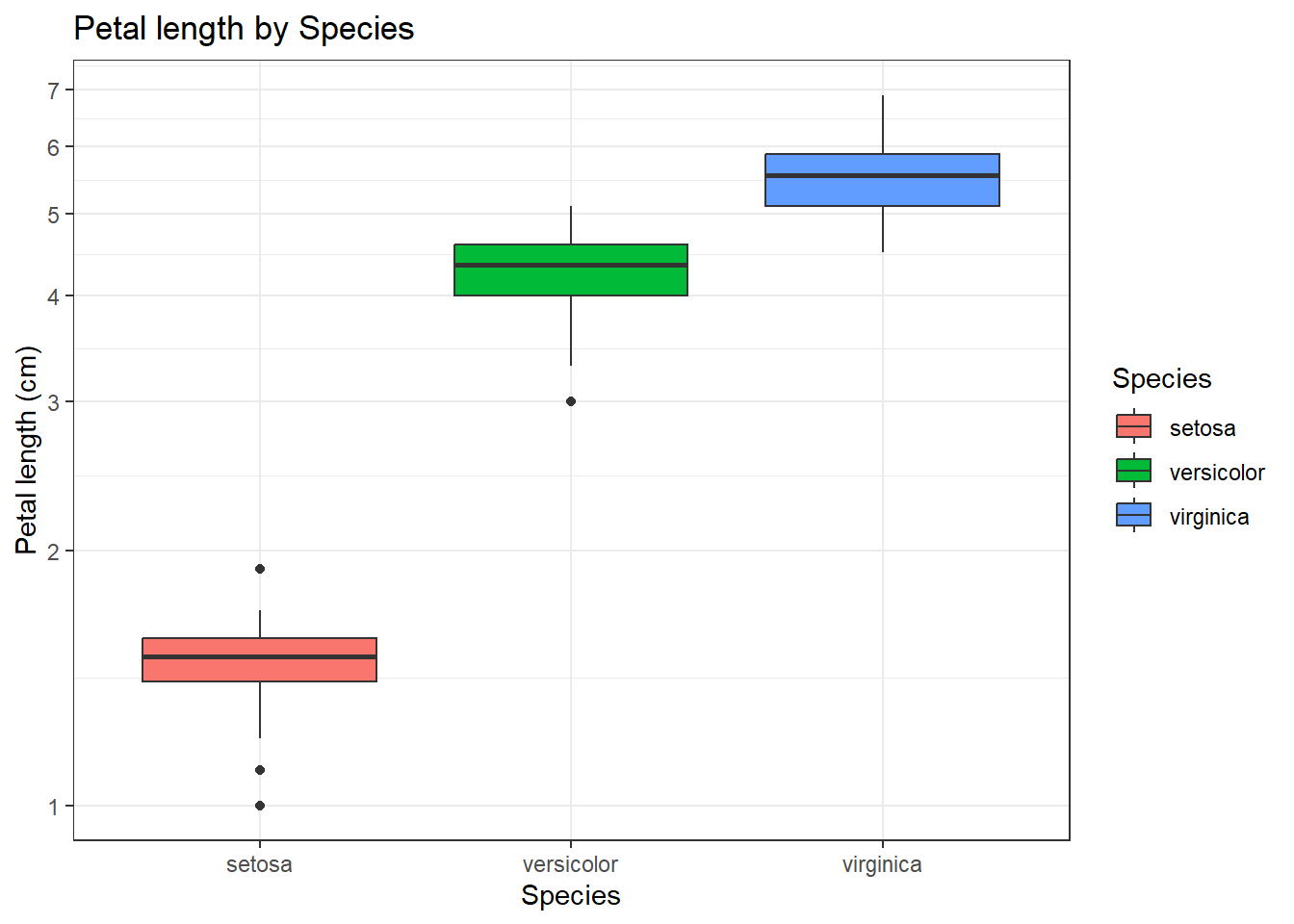

If we want to export the plot we can assign it to an object then save that object with ggsave:

boxplot1 <- ggplot(iris) + 
  aes(x=Species , y=Petal.Length, fill=Species) + 
  geom_boxplot()
ggsave("lengthboxplot.png",boxplot1, width=5, height=5, dpi="retina")

I was asked what would happen if we wanted to load data with no header. The best answer is ‘try it and see’. We make iris2.csv with no header row. When we tried to load it, the first row of values was assumed to be the header.

iris2 <- read.csv("iris2.csv")
head(iris2)

  X1 X5.1 X3.5 X1.4 X0.2 setosa
1  2  4.9  3.0  1.4  0.2 setosa
2  3  4.7  3.2  1.3  0.2 setosa
3  4  4.6  3.1  1.5  0.2 setosa
4  5  5.0  3.6  1.4  0.2 setosa
5  6  5.4  3.9  1.7  0.4 setosa
6  7  4.6  3.4  1.4  0.3 setosa

So we looked at the help file to check how to correctly load the data, and how to assign names if we wanted to.

iris2 <- read.csv(file = "iris2.csv",
                  header=FALSE,
                  col.names = c("X", "PL", "PW", "SW", "SL", "Species"))
head(iris2)

  X  PL  PW  SW  SL Species
1 1 5.1 3.5 1.4 0.2  setosa
2 2 4.9 3.0 1.4 0.2  setosa
3 3 4.7 3.2 1.3 0.2  setosa
4 4 4.6 3.1 1.5 0.2  setosa
5 5 5.0 3.6 1.4 0.2  setosa
6 6 5.4 3.9 1.7 0.4  setosa

3 Modelling

Most of our statistical tests can be thought of in terms of statistical models. Simple linear regression models are the simplest models, we can do most things by generalisaing these.

In R, we use a formula to describe the model we want to estimate. Here we want to model how the average of sepal width varies (statistically, not necessarily causally) with sepal length.

lm(data=iris , Sepal.Width ~ Sepal.Length)


Call:
lm(formula = Sepal.Width ~ Sepal.Length, data = iris)

Coefficients:
 (Intercept)  Sepal.Length  
     3.41895      -0.06188

To do anything useful we need to make an lm object (here called model1)

model1 <- lm(data=iris , Sepal.Width ~ Sepal.Length)

Now we extract the model summary

summary(model1)


Call:
lm(formula = Sepal.Width ~ Sepal.Length, data = iris)

Residuals:
    Min      1Q  Median      3Q     Max 
-1.1095 -0.2454 -0.0167  0.2763  1.3338 

Coefficients:
             Estimate Std. Error t value Pr(>|t|)    
(Intercept)   3.41895    0.25356   13.48   <2e-16 ***
Sepal.Length -0.06188    0.04297   -1.44    0.152    
---
Signif. codes:  0 '***' 0.001 '**' 0.01 '*' 0.05 '.' 0.1 ' ' 1

Residual standard error: 0.4343 on 148 degrees of freedom
Multiple R-squared:  0.01382,   Adjusted R-squared:  0.007159 
F-statistic: 2.074 on 1 and 148 DF,  p-value: 0.1519

Get the gtsummary package if you don’t have it already. (with install.packages("gtsummary")).
The tbl_regression function from this package makes a nicely formatted regression table.

gtsummary::tbl_regression(model1)

Characteristic	Beta	95% CI¹	p-value
Sepal.Length	-0.06	-0.15, 0.02	0.2
¹ CI = Confidence Interval

We can also use ggplot to draw a linear model: Note how the slope and intercept of the stat_smooth line corresponds to the model summary output

iris |> ggplot() + 
  aes(x=Sepal.Length , 
      y=Sepal.Width, 
      ) + 
  geom_point() +
  theme_bw() +
  stat_smooth(method="lm")

`geom_smooth()` using formula = 'y ~ x'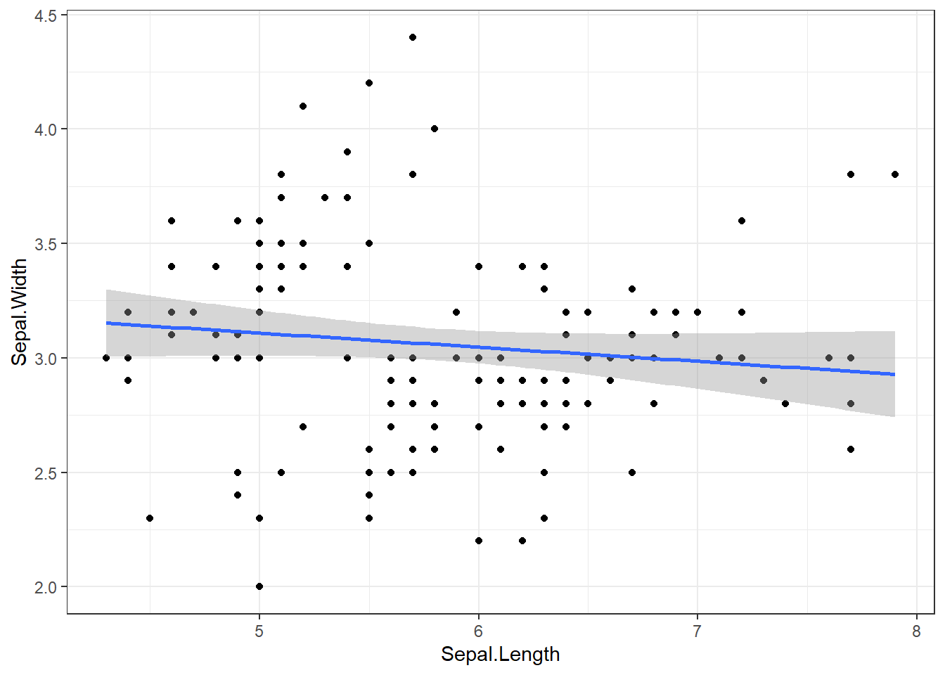

By adding colours we can see that our first model may not be the best, because there is clearly an effect of species on the outcome variable that we have ignored. So we should estimate a separate line for each species, but consider that we have changed the reserach question quite substantially:

iris |> ggplot() + 
  aes(x=Sepal.Length , 
      y=Sepal.Width, 
      shape=Species,
      col=Species) + 
  geom_point() +
  theme_bw() +
  stat_smooth(method="lm")

`geom_smooth()` using formula = 'y ~ x'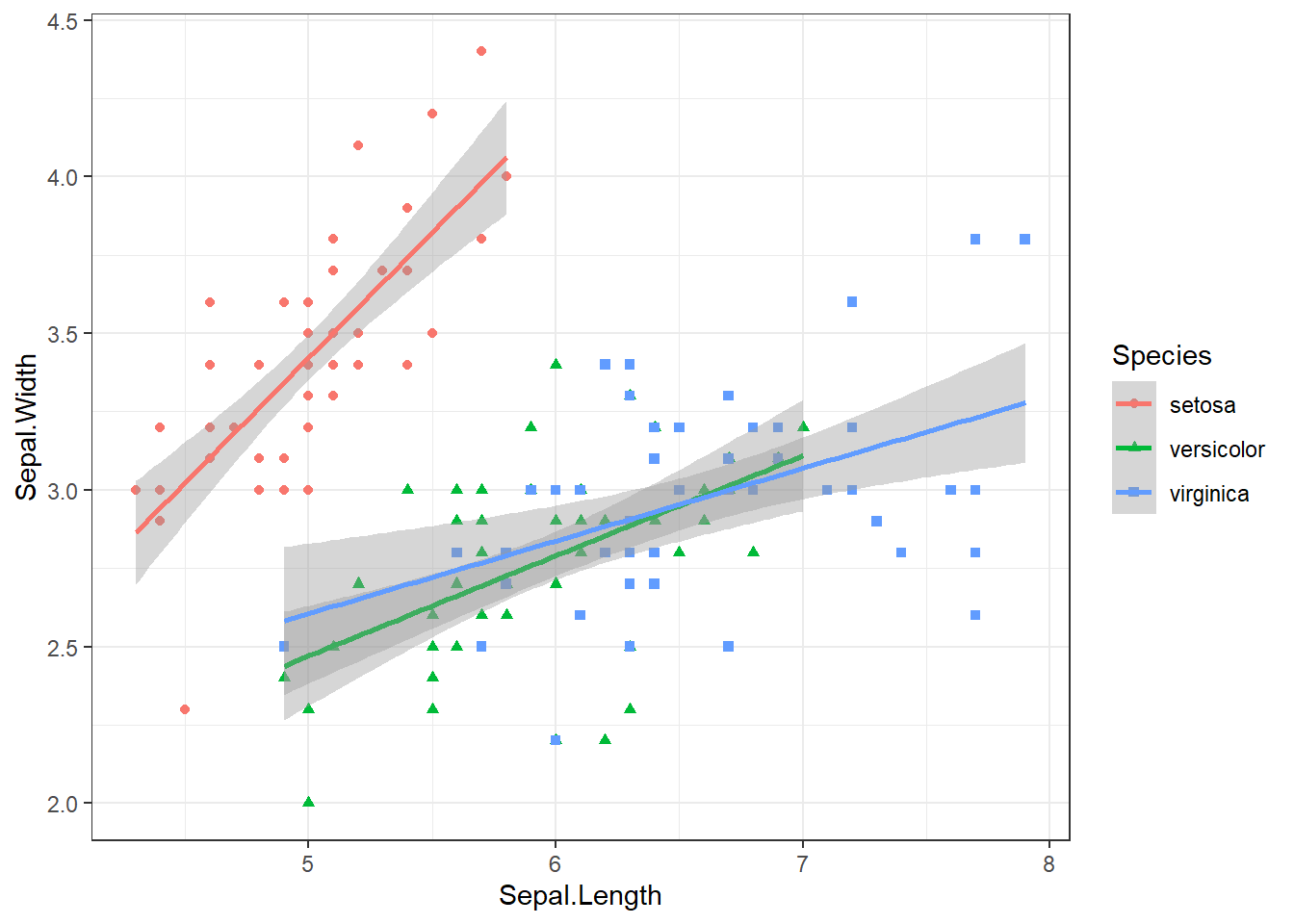

We can make linear models corresponding to more complex relationships! This is an advantage of using linear models instead of other ‘ad hoc’ statistical testing. This model corrects for the effect of species on sepal width:

Entering just the main effect (as below) lead to a separate but parallel line for each species. The slope (effect of sepal length) does not vary with species.

model2 <- lm(data = iris , Sepal.Width ~ Sepal.Length + Species )
summary(model2)


Call:
lm(formula = Sepal.Width ~ Sepal.Length + Species, data = iris)

Residuals:
     Min       1Q   Median       3Q      Max 
-0.95096 -0.16522  0.00171  0.18416  0.72918 

Coefficients:
                  Estimate Std. Error t value Pr(>|t|)    
(Intercept)        1.67650    0.23536   7.123 4.46e-11 ***
Sepal.Length       0.34988    0.04630   7.557 4.19e-12 ***
Speciesversicolor -0.98339    0.07207 -13.644  < 2e-16 ***
Speciesvirginica  -1.00751    0.09331 -10.798  < 2e-16 ***
---
Signif. codes:  0 '***' 0.001 '**' 0.01 '*' 0.05 '.' 0.1 ' ' 1

Residual standard error: 0.289 on 146 degrees of freedom
Multiple R-squared:  0.5693,    Adjusted R-squared:  0.5604 
F-statistic: 64.32 on 3 and 146 DF,  p-value: < 2.2e-16

But we can add an interaction term to allow the effect of sepal length to vary by species These two models are the same.

model4 <- lm(data = iris , Sepal.Width ~ Sepal.Length + Species + Sepal.Length:Species )
model4 <- lm(data = iris , Sepal.Width ~ Sepal.Length * Species )
summary(model4)


Call:
lm(formula = Sepal.Width ~ Sepal.Length * Species, data = iris)

Residuals:
     Min       1Q   Median       3Q      Max 
-0.72394 -0.16327 -0.00289  0.16457  0.60954 

Coefficients:
                               Estimate Std. Error t value Pr(>|t|)    
(Intercept)                     -0.5694     0.5539  -1.028 0.305622    
Sepal.Length                     0.7985     0.1104   7.235 2.55e-11 ***
Speciesversicolor                1.4416     0.7130   2.022 0.045056 *  
Speciesvirginica                 2.0157     0.6861   2.938 0.003848 ** 
Sepal.Length:Speciesversicolor  -0.4788     0.1337  -3.582 0.000465 ***
Sepal.Length:Speciesvirginica   -0.5666     0.1262  -4.490 1.45e-05 ***
---
Signif. codes:  0 '***' 0.001 '**' 0.01 '*' 0.05 '.' 0.1 ' ' 1

Residual standard error: 0.2723 on 144 degrees of freedom
Multiple R-squared:  0.6227,    Adjusted R-squared:  0.6096 
F-statistic: 47.53 on 5 and 144 DF,  p-value: < 2.2e-16

We can use the emmeans package to extract the slope at each level of Species from model 4.

emmeans::emtrends(model4 , pairwise~Species , var="Sepal.Length")

$emtrends
 Species    Sepal.Length.trend     SE  df lower.CL upper.CL
 setosa                  0.799 0.1104 144    0.580    1.017
 versicolor              0.320 0.0754 144    0.171    0.469
 virginica               0.232 0.0612 144    0.111    0.353

Confidence level used: 0.95 

$contrasts
 contrast               estimate     SE  df t.ratio p.value
 setosa - versicolor      0.4788 0.1337 144   3.582  0.0013
 setosa - virginica       0.5666 0.1262 144   4.490  <.0001
 versicolor - virginica   0.0878 0.0971 144   0.905  0.6382

P value adjustment: tukey method for comparing a family of 3 estimates

The ANOVA function can be used to generate the old-fashioned ANOVA table corresponding to each model:

anova(model4)

Analysis of Variance Table

Response: Sepal.Width
                      Df  Sum Sq Mean Sq  F value    Pr(>F)    
Sepal.Length           1  0.3913  0.3913   5.2757   0.02307 *  
Species                2 15.7225  7.8613 105.9948 < 2.2e-16 ***
Sepal.Length:Species   2  1.5132  0.7566  10.2011  7.19e-05 ***
Residuals            144 10.6800  0.0742                       
---
Signif. codes:  0 '***' 0.001 '**' 0.01 '*' 0.05 '.' 0.1 ' ' 1

Or to test whether one model is a significantly better fit than another:

anova(model1 , model2, model4)

Analysis of Variance Table

Model 1: Sepal.Width ~ Sepal.Length
Model 2: Sepal.Width ~ Sepal.Length + Species
Model 3: Sepal.Width ~ Sepal.Length * Species
  Res.Df    RSS Df Sum of Sq       F    Pr(>F)    
1    148 27.916                                   
2    146 12.193  2   15.7225 105.995 < 2.2e-16 ***
3    144 10.680  2    1.5132  10.201  7.19e-05 ***
---
Signif. codes:  0 '***' 0.001 '**' 0.01 '*' 0.05 '.' 0.1 ' ' 1

Here we see model 4 is better than model 2, (and model 2 is better than model 1). So there is good evidence that we should fit independent slopes for each species.

4 Some linear algebra

I was asked about the maths underlying the linear regression.
Linear Algebra for linear regression is straightforward, and is explained here (https://xebia.com/blog/the-linear-algebra-behind-linear-regression/).
Most of you will not need to worry about this! You can calculate the coefficients by extracting the model matrix, then applying the following formula:

X <- model.matrix(model2)
b = solve(t(X)%*%X) %*% 
  t(X) %*% 
  iris$Sepal.Width
b

                        [,1]
(Intercept)        1.6765001
Sepal.Length       0.3498801
Speciesversicolor -0.9833885
Speciesvirginica  -1.0075104

Compare it to:

coef(model2)

      (Intercept)      Sepal.Length Speciesversicolor  Speciesvirginica 
        1.6765001         0.3498801        -0.9833885        -1.0075104

Get the residual error

sigma <- ((X %*% b - iris$Sepal.Width) |> sd())*sqrt((149/146))
sigma

[1] 0.288989

compare it to:

sigma(model2)

[1] 0.288989

5 Day 3 script - a bit more analysis, ANOVA and log-transformation

On day three we looked at a few different graphs:

library(ggplot2)
library(ggbeeswarm)

Warning: package 'ggbeeswarm' was built under R version 4.3.3

A box plot shows a great ‘five point summary’ for each distribution

ggplot(iris) + aes(x=Species, y=Petal.Length, fill=Species) + 
  geom_boxplot(outlier.colour = NA) + 
  geom_beeswarm(size=1)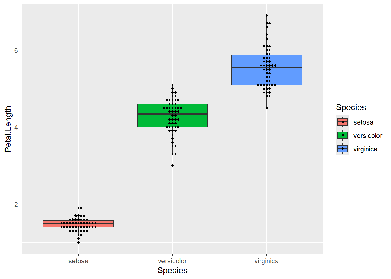

The log-scale graph suggested that a log-transformed model might be more appropriate

ggplot(iris) + aes(x=Species, y=Petal.Length, fill=Species) + 
  geom_boxplot(outlier.colour = NA) + 
  geom_beeswarm(size=1) + 
  scale_y_log10()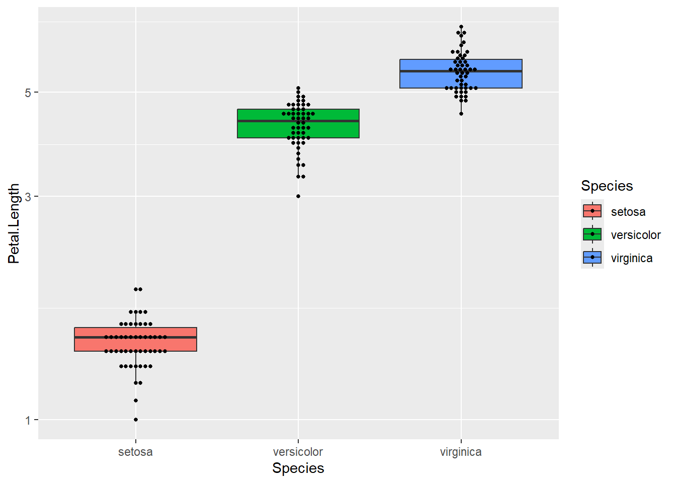

A ‘dynamite’ plot is less useful, but could be acceptable if you overlay the true data points.

ggplot(iris) + aes(x=Species, y=Petal.Length, fill=Species) + 
  stat_summary(geom="col") + 
  stat_summary(geom="errorbar", width=0.5) + 
  geom_beeswarm()

No summary function supplied, defaulting to `mean_se()`
No summary function supplied, defaulting to `mean_se()`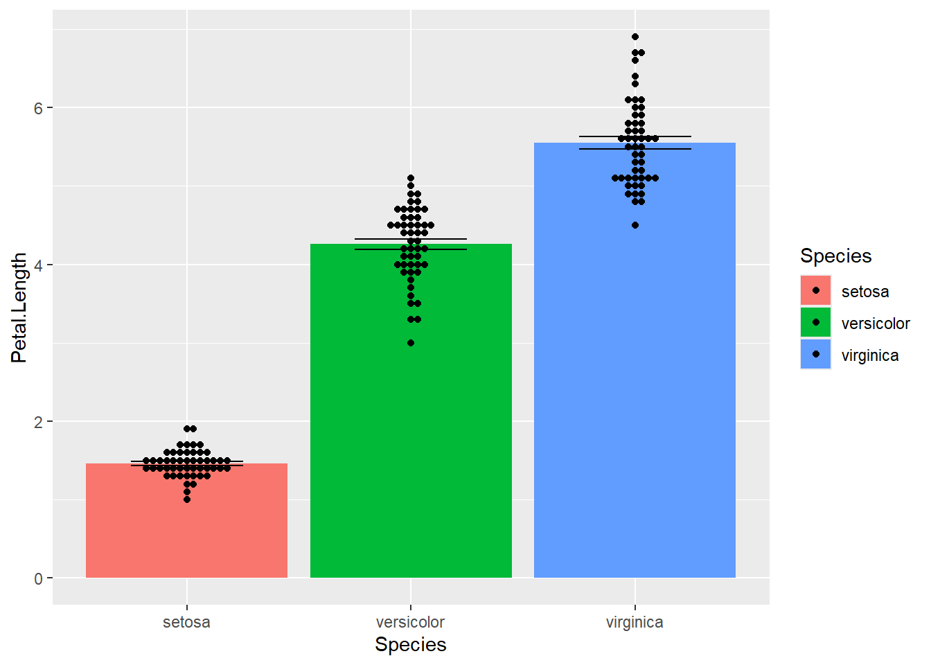

We can estimate a model corresponding to these graphs. The 1+ tells R to include an intercept term. We don’t need to explicity say this, but if we don’t want the intercept then we need to use 0+.

model_petal_length_species <- lm(data=iris , Petal.Length ~ 1+Species)

This is an anova for the hypothesis that all the species differences are zero

anova(model_petal_length_species)

Analysis of Variance Table

Response: Petal.Length
           Df Sum Sq Mean Sq F value    Pr(>F)    
Species     2 437.10 218.551  1180.2 < 2.2e-16 ***
Residuals 147  27.22   0.185                      
---
Signif. codes:  0 '***' 0.001 '**' 0.01 '*' 0.05 '.' 0.1 ' ' 1

The model summary shows the individual regression coefficients

summary(model_petal_length_species)


Call:
lm(formula = Petal.Length ~ 1 + Species, data = iris)

Residuals:
   Min     1Q Median     3Q    Max 
-1.260 -0.258  0.038  0.240  1.348 

Coefficients:
                  Estimate Std. Error t value Pr(>|t|)    
(Intercept)        1.46200    0.06086   24.02   <2e-16 ***
Speciesversicolor  2.79800    0.08607   32.51   <2e-16 ***
Speciesvirginica   4.09000    0.08607   47.52   <2e-16 ***
---
Signif. codes:  0 '***' 0.001 '**' 0.01 '*' 0.05 '.' 0.1 ' ' 1

Residual standard error: 0.4303 on 147 degrees of freedom
Multiple R-squared:  0.9414,    Adjusted R-squared:  0.9406 
F-statistic:  1180 on 2 and 147 DF,  p-value: < 2.2e-16

We can get the pairwise contrasts with emmeans.

emmeans::emmeans(model_petal_length_species , pairwise ~ Species)

$emmeans
 Species    emmean     SE  df lower.CL upper.CL
 setosa       1.46 0.0609 147     1.34     1.58
 versicolor   4.26 0.0609 147     4.14     4.38
 virginica    5.55 0.0609 147     5.43     5.67

Confidence level used: 0.95 

$contrasts
 contrast               estimate     SE  df t.ratio p.value
 setosa - versicolor       -2.80 0.0861 147 -32.510  <.0001
 setosa - virginica        -4.09 0.0861 147 -47.521  <.0001
 versicolor - virginica    -1.29 0.0861 147 -15.012  <.0001

P value adjustment: tukey method for comparing a family of 3 estimates

We said the log-transformation might be needed. We can estimate a model for log(Petal.Length)

model_petal_length_species_log <- 
  lm(data=iris , log(Petal.Length) ~ Species)

Now emmeans reports ratios instead of differences. Could make more sense biologically!

emmeans::emmeans(model_petal_length_species_log , 
                 pairwise ~ Species, type="response")

$emmeans
 Species    response     SE  df lower.CL upper.CL
 setosa         1.45 0.0230 147     1.41     1.50
 versicolor     4.23 0.0670 147     4.10     4.37
 virginica      5.53 0.0874 147     5.36     5.70

Confidence level used: 0.95 
Intervals are back-transformed from the log scale 

$contrasts
 contrast               ratio      SE  df null t.ratio p.value
 setosa / versicolor    0.343 0.00767 147    1 -47.835  <.0001
 setosa / virginica     0.263 0.00588 147    1 -59.747  <.0001
 versicolor / virginica 0.766 0.01714 147    1 -11.912  <.0001

P value adjustment: tukey method for comparing a family of 3 estimates 
Tests are performed on the log scale