set.seed(1)
populationsize = 1e4
samplesize = 200

population <- data.frame(health=rnorm(populationsize), wealth=rnorm(populationsize))
plot(population)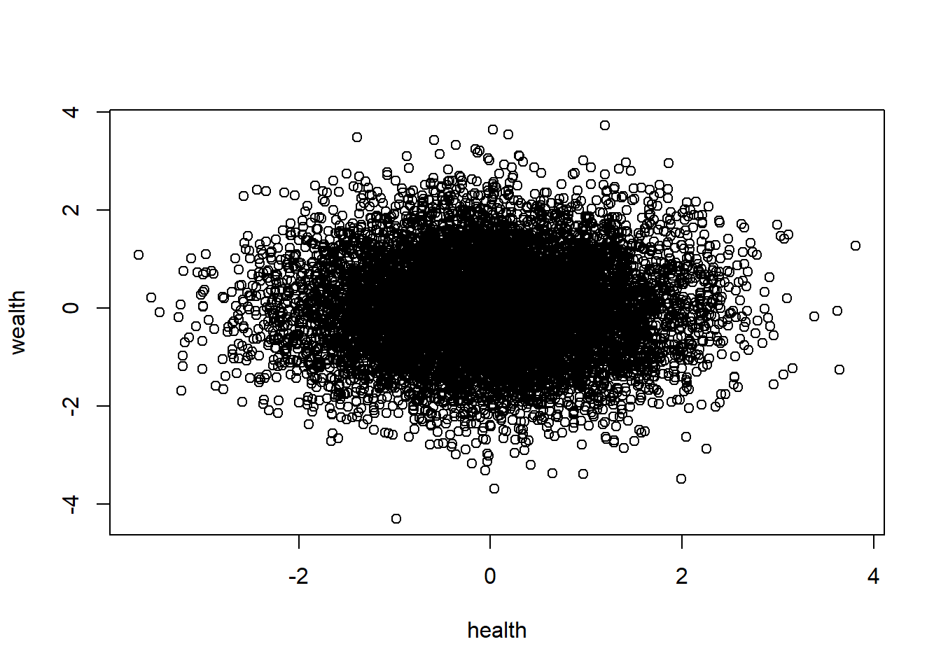
George Savva, (QIB)
This is a short illustration of “Berkson bias” using simulated data. This is the phenomenon that selection bias can induce correlations in samples that are not present in populations.
This bias is likely to be an issue for many observational studies but is not well understood in the medical research literature.
The Wikipedia page for the phenonomenon is here: https://en.wikipedia.org/wiki/Berkson%27s_paradox
Suppose we are trying to understand the correlation between health and wealth.
First, let’s simulation a population in which health and wealth are both normally distributed but are not correlated with each other:
set.seed(1)
populationsize = 1e4
samplesize = 200
population <- data.frame(health=rnorm(populationsize), wealth=rnorm(populationsize))
plot(population)
Now if we take a simple random sample from this cohort from this group and test the correlation…
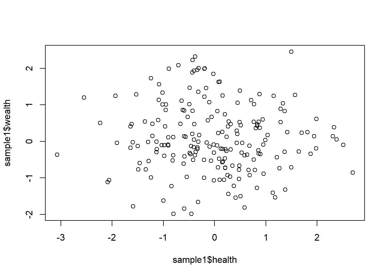
    Pearson's product-moment correlation

data:  sample1$health and sample1$wealth
t = -0.78426, df = 198, p-value = 0.4338
alternative hypothesis: true correlation is not equal to 0
95 percent confidence interval:
 -0.19290026  0.08373896
sample estimates:
        cor
-0.05564858
We see no evidence that wealth and health are related, as we would expect given this is true in the population.
However we know that healthier, wealthier people are more likely to participate in our studies. So let’s create a sample that reflects this:
How will the average health and wealth in our sample compare to the population?
Well we know that health and wealth are higher in the sample than the population, but this should hopefullt be obvious. But how are the two things correlated in the population?
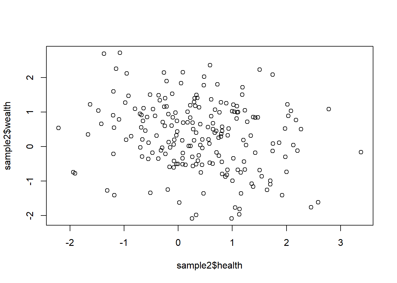
    Pearson's product-moment correlation

data:  sample2$health and sample2$wealth
t = -2.9629, df = 198, p-value = 0.003421
alternative hypothesis: true correlation is not equal to 0
95 percent confidence interval:
 -0.3352015 -0.0692823
sample estimates:
       cor
-0.2060428
It looks like a negative correlation in the sample, despite there being no correlation in the population!
Was this unlucky? We can look at the distribution of p-values from repeated samples, to see what the chance of a false positive correlation is here:
onepvalue <- function(){
  samplen <- population[sample(populationsize, samplesize, prob = population$prob_participate),]
  cor.test(samplen$health, samplen$wealth)$p.value
}
replicate(1000, onepvalue()) |> hist(breaks=20)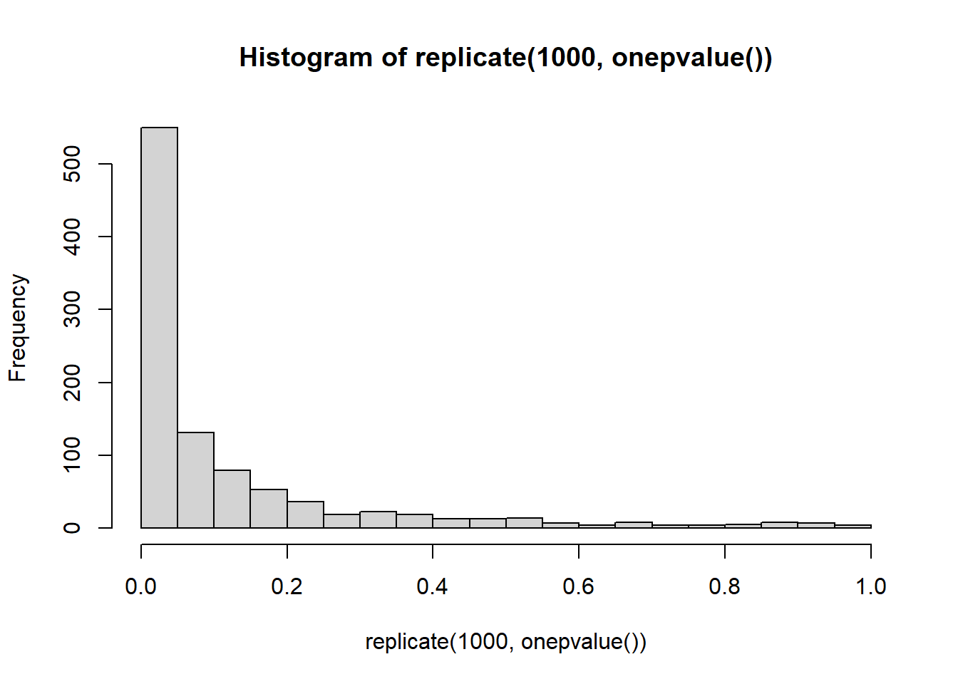
In more than 50% of cases there is now a significant correlation in the sample even though there is no correlation in the population. It is simply caused by the factors under investigation also being factors that lead people to participate in research.
What are the implications of this for observational studies?
What can we do about it? If we have sampling weights it is relatively easy to fix, but what if we don’t? Do we have to try to get them somehow?