Descriptive tables using base R, data.table and tidyverse

Author

George Savva

Published

October 2, 2023

Limitations of “base” R

With only base R (that is, R without add on packages) it can be unexpectedly difficult to perform some simple tasks.

A good example is making a table of summary statistics. This is difficult with base R but is simple with using function from add-on packages.

Here I illustrate this using two widely used systems for data manipulation in R, namely data.table and tidyverse. Both can be used to make summary tables of descriptive statistics. that can be exported

Finally I describe a package, gtsummary that is specifically designed for creation of publication ready summary tables.

Mean of one variable stratified by another

Suppose we have a dataset of the heights (in cm) of 100 men and women, and we want to make a descriptive table of means, standard deviations and counts by sex.

First let’s make a fake dataset. We’ll assume women have an average height of 170cm, men of 180cm with both groups normally distributed with a standard deviation of 10.

# Look up 'sample' to understand what this does
sex = sample(c("Male", "Female"), size=100, replace=TRUE)

# What does this line do?
height = rnorm(n=100, 
               mean=180 + 10* (sex=="Male"), 
               sd=10)

# We have two vectors of the same length so we can combine them into a data frame.
dat = data.frame(height,sex)

Now lets quickly check the data using a plot to make sure it looks as we would expect.

head(dat)

    height    sex
1 202.6168   Male
2 189.1209   Male
3 189.6766   Male
4 175.0141 Female
5 184.4425 Female
6 172.5497 Female

boxplot(dat$height~dat$sex)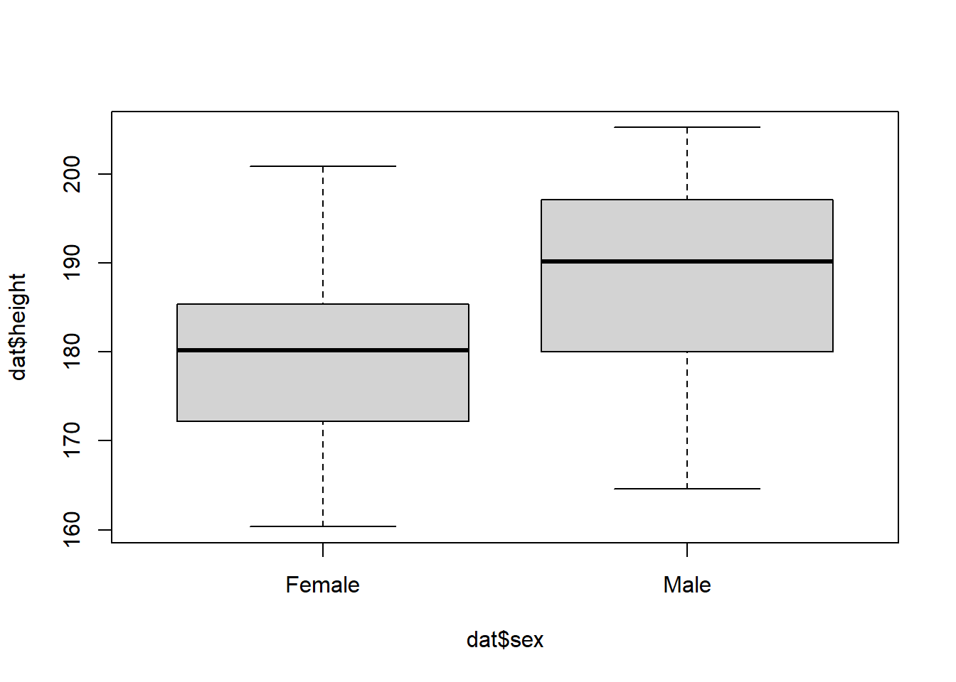

The base R way to get summary statistics

The aggregate function can be used to calculate a single statistic over groups as follows:

aggregate( height ~ sex , FUN=mean, data=dat)

     sex   height
1 Female 179.1283
2   Male 191.0083

Alternatively we could use tapply:

tapply( dat$height, dat$sex , FUN=mean )

  Female     Male 
179.1283 191.0083

While this works in this simple case it is difficult to get a more complicated table. For example, there is no obvious way to get a table of means, standard deviations and counts (the standard table 1 in any biomedical paper) without using an external package.

I’ll illustrate three different approaches of here. First, data.table and tidyverse add ways to manage and manipulate data

It is likely that if you spend a lot of time using R you should learn to use one or other (or both) of these systems.

Then I’ll illustrate gtsummary, a package specifically designed to make tabulation of results easier.

Using `data.table`

The data.table package gives us a very flexible way to perform fast grouped operations on datasets. A data.table is an enhanced version of a data.frame, and the main function of data.table an extension to the [ ] operator (square brackets) that is much more powerful than the default R version.

First we need to load the package, then turn the data.frame into a data.table using setDT.

library(data.table) # Load the package

Warning: package 'data.table' was built under R version 4.3.3

setDT(dat)          # Turn our "data frame" 'dat' into a "data table"

Now we can use the extended square bracket syntax to create our table.

First the simple comparison of means:

dat[ , mean(height), by=sex ]

      sex       V1
   <char>    <num>
1:   Male 191.0083
2: Female 179.1283

Next, adding the counts and standard deviations:

dat[ , .(Count=.N, Mean=mean(height),SD=sd(height)), by=sex]

      sex Count     Mean        SD
   <char> <int>    <num>     <num>
1:   Male    56 191.0083 10.751836
2: Female    44 179.1283  9.081369

Breaking down the data.table syntax

The [ operator in data.table has three arguments. In short, we express a command on a dataset (here called dat) by specifying:

dat[ which rows to use , what to do , which columns to group on ]

In the first version of the command above we left the first entry blank (so used all the rows), placed mean(height) in the second position and specified by=sex in the third. In the second version we expanded the second argument to return a list of elements, and gave them new names.

For more details of using data.table, see: https://cran.r-project.org/web/packages/data.table/vignettes/datatable-intro.html

The `tidyverse` way

tidyverse is a set of R packages that provide many functions for data manipulation and programming. In particular the dplyr library includes functions for data manipulation and summarisation. To use these we can load the dplyr library:

library(dplyr)


Attaching package: 'dplyr'

The following objects are masked from 'package:data.table':

    between, first, last

The following objects are masked from 'package:stats':

    filter, lag

The following objects are masked from 'package:base':

    intersect, setdiff, setequal, union

Then get our results table the tidyverse way:

First just the means

dat %>% group_by(sex) %>% summarise(mean(height))

# A tibble: 2 × 2
  sex    `mean(height)`
  <chr>           <dbl>
1 Female           179.
2 Male             191.

Now with the counts and standard deviations:

dat %>% group_by(sex) %>% summarise(N=n(),mean(height), sd(height))

# A tibble: 2 × 4
  sex        N `mean(height)` `sd(height)`
  <chr>  <int>          <dbl>        <dbl>
1 Female    44           179.         9.08
2 Male      56           191.        10.8

The tidyverse (dplyr) syntax

dplyr introduces six main functions for manipulating and summarising data, these are mutate, arrange, select, filter, summarise, and group_by. Using combinations of these functions you can perform most simple data operations. Functions are chained together using the pipe operator %>% which passes the output from one into the next.

So the first command above reads something like: “take dat, then group it by sex, then for each group return the summary statistics we specified”.

Visit https://www.tidyverse.org/learn for more.

Using `gtsummary`

Finally to illustrate a package meant specifically for nicely formatted data tabulations, the tbl_summary function from the gtsummary package can create tables of descriptives. gtsummary is built on the gt package, a part of the tidyverse which provides visual formatting for tables, analogous to ggplot2 for graphs.

library(gtsummary)
tbl_summary(dat, by=sex, statistic=list(height~"{mean} ({sd})"))

Characteristic	Female N = 44¹	Male N = 56¹
height	179 (9)	191 (11)
¹ Mean (SD)

This is a little different to the other approaches, because it produces a publication ready output rather than a dataset for further processing as do

https://www.rdocumentation.org/packages/gtsummary/versions/1.6.3

Which to use?

data.table and tidyverse perform a lot of the same tasks in improving the R experience. You will probably choose to mainly use one or the other (or to mostly stick with base R), but it will help to be familiar with both if you want to understand and reuse code written by others.

If you search tidyverse vs data.table online you will find a lot of differing opinions as to which to use. More people learn tidyverse now, possibly because it has a lot of resources put into its development and promotion.

Personally I like the data.table syntax better so I tend to use this, borrowing from tidyverse packages when I need to. I find that the more confident I get with it, the more data.table features I use, which I think improves my code.

The gt system for making nice tables is popular with people making reports and is well integrated into the tidyverse ecosystem.

Limitations of “base” R

Mean of one variable stratified by another

The base R way to get summary statistics

Using data.table

Breaking down the data.table syntax

The tidyverse way

The tidyverse (dplyr) syntax

Using gtsummary

Which to use?

Further reading

Using `data.table`

The `tidyverse` way

Using `gtsummary`